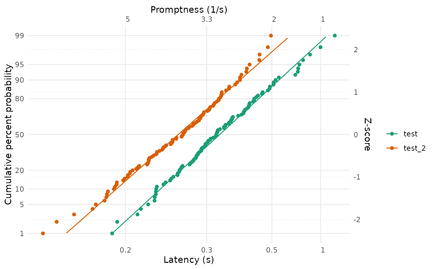
Plot reaction times and LATER model fit in reciprobit axes

Usage

reciprobit_plot(
  plot_data,
  fit_params = NULL,
  time_breaks = c(0.1, 0.2, 0.3, 0.5, 1),
  probit_breaks = c(0.1, 1, 5, 10, 20, 50, 80, 90, 95, 99, 99.9),
  z_breaks = c(-2, -1, 0, 1, 2),
  xrange = NULL,
  yrange = NULL
)

Arguments

plot_data: A dataframe with columns: time, name, promptness, and e_cdf. Optionally, there may be a color column, which contains hex values, one unique hex value per named dataset
fit_params: A dataframe with one row for each named dataset and columns equal to the LATER model parameters returned by fit_data$named_fit_params
time_breaks: Desired tick marks on the x axis, expressed in promptness (1/s)
probit_breaks: Desired tick marks on the y axis in probit space
z_breaks: Desired tick marks on secondary y axis, in z values
xrange: Desired range for the x axis, in promptness (1/s)
yrange: Desired range for the y axis, in cumulative probability space

Value

A reciprobit plot with the cumulative probability distribution of the reaction times

Examples

# \donttest{
data <- rbind(
  data.frame(name = "test", time = 1000/rnorm(100, 3, 1)),
  data.frame(name = "test_2", time = 1000/rnorm(100, 4, 1))
) |> dplyr::filter(time > 0)
data <- prepare_data(data)
fit_params <- individual_later_fit(data)
reciprobit_plot(data, fit_params)

# }