Analysis of 'Neural computation of log likelihood in control of saccadic eye movements'

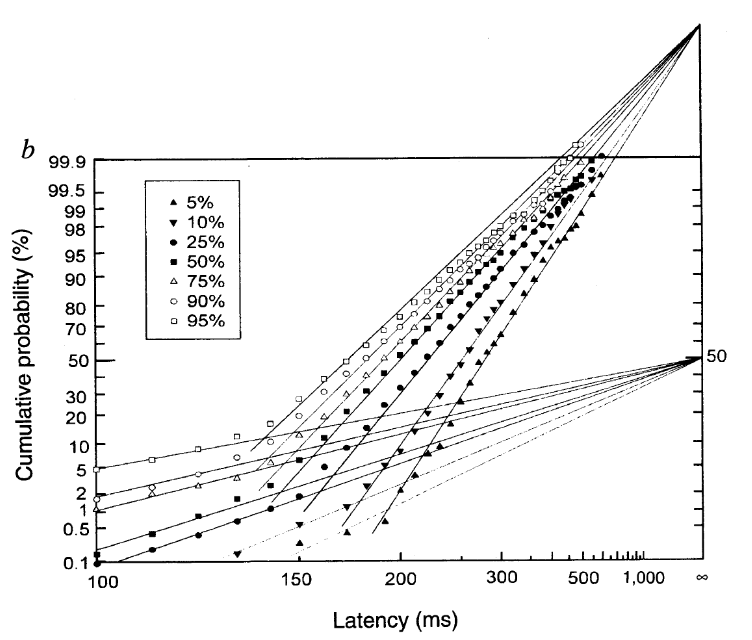
Here, we will walk through the analysis of some example data from the article “Neural computation of log likelihood in control of saccadic eye movements” by Carpenter and Williams (1995). We will be particularly interested in analysing the data from participant b, as shown in the figure below (their Figure 2b).

We will be looking at how we can use the LATERmodel package to load, fit, visualise, and evaluate data in the context of the LATER model of response times. If the LATERmodel package has not yet been installed, it can be installed by running the following within R:

install.packages("LATERmodel")

Loading the raw data

A digitised version of the raw data from this study is included in this package in the LATERmodel::carpenter_williams_1995 variable. This variable is a dataframe with rows corresponding to trials and with columns named participant, condition, and time. This is the recommended format for raw data to be used with the LATERmodel package. The participant and condition columns specify the identifiers for the participant and condition, respectively, and the time column specifies the measured response time (in milliseconds). The rows corresponding to a particular unique combination of participant and condition are referred to as a dataset within this package.

We can look at the first few rows, using the head function, to see the structure of the dataframe:

head(LATERmodel::carpenter_williams_1995)

participant	condition	time
a	p95	100
a	p95	100
a	p95	100
a	p95	100
a	p95	100
a	p95	100

Because LATERmodel::carpenter_williams_1995 contains trials for both participants a and b but we are only interested in participant b here, we will extract only the trials for participant b from this variable using the subset function:

raw_data <- subset(x = LATERmodel::carpenter_williams_1995, participant == "b")

Pre-processing the data

The data analysis functions within this LATERmodel package require the raw data to first undergo pre-processing using the LATERmodel::prepare_data function. We pass our raw_data variable as the argument to the raw_data parameter of LATERmodel::prepare_data to perform such pre-processing:

data <- LATERmodel::prepare_data(raw_data = raw_data)

Note that if the raw data had response times in units other than milliseconds, we could have used the time_unit parameter to LATERmodel::prepare_data to specify the units (see the documentation for LATERmodel::prepare_data for details).

We can again view the first few rows to inspect the output of the pre-processing:

head(data)
#> # A tibble: 6 × 4
#> # Groups:   name [1]
#>    time name  promptness e_cdf
#>   <dbl> <fct>      <dbl> <dbl>
#> 1  0.15 b_p05       6.67 0.998
#> 2  0.17 b_p05       5.88 0.996
#> 3  0.19 b_p05       5.26 0.992
#> 4  0.19 b_p05       5.26 0.992
#> 5  0.2  b_p05       5    0.977
#> 6  0.2  b_p05       5    0.977

As shown above, the data now has columns for name (formed from the combination of the participant and condition columns in the raw data), promptness (the inverse of the time column, which is now specified in seconds), and e_cdf (the evaluated empirical cumulative distribution function for each dataset).

To make the condition names match those used in Carpenter and Williams (1995), we can recode them:

# make the names match C&W
data$name <- dplyr::recode_factor(
  .x = data$name,
  b_p05 = "5%",
  b_p10 = "10%",
  b_p25 = "25%",
  b_p50 = "50%",
  b_p75 = "75%",
  b_p90 = "90%",
  b_p95 = "95%"
)

Visualising the observed data

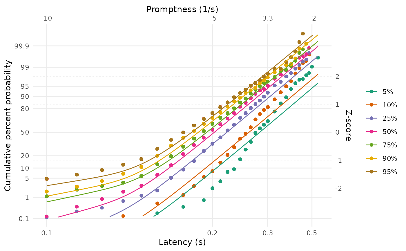
We can use the LATERmodel::reciprobit_plot function to visualise the observed data in ‘reciprobit’ space:

LATERmodel::reciprobit_plot(plot_data = data)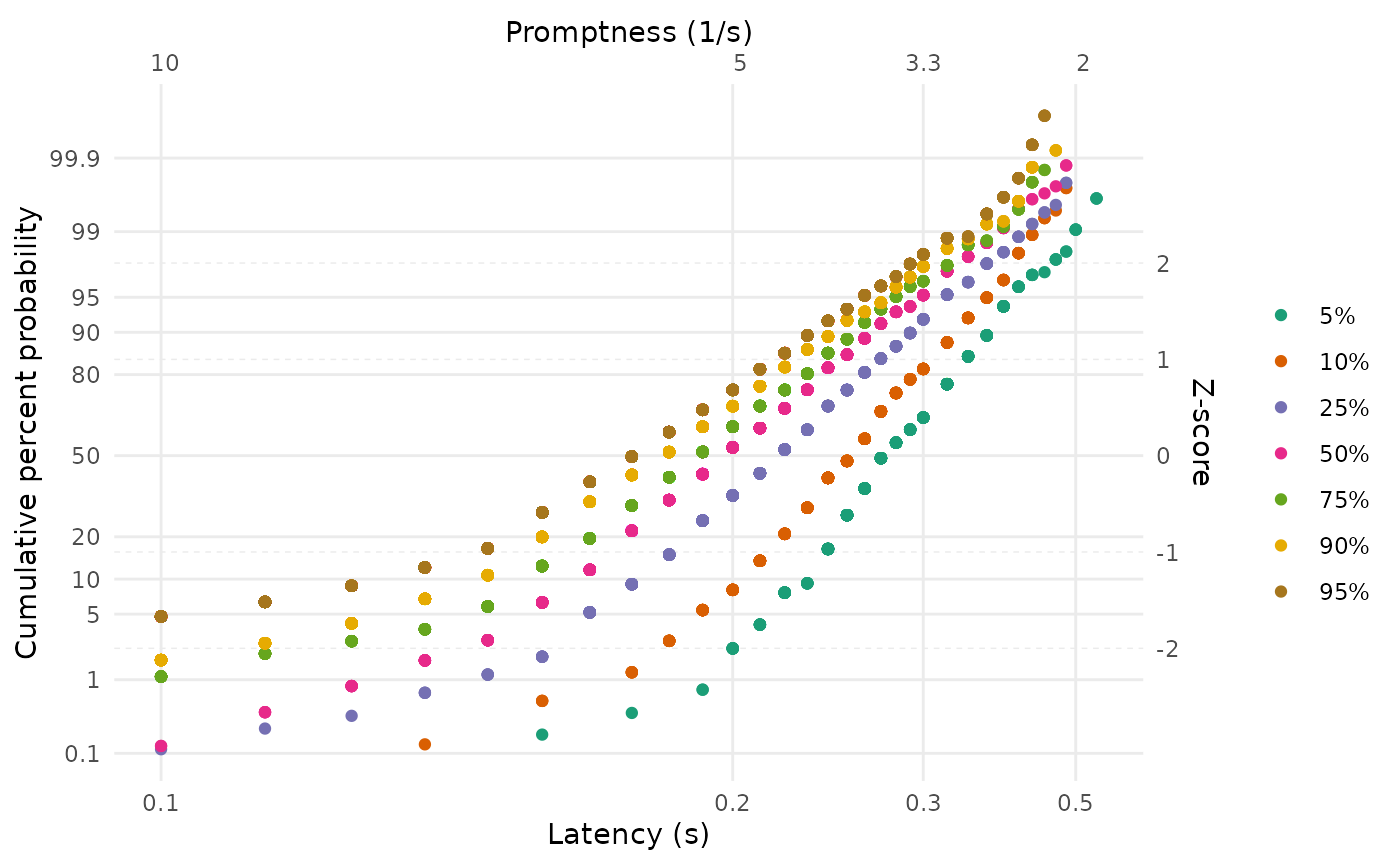

This produces a plot in which the empirical cumulative distribution function values for each of the datasets in data are shown as individual points, with points from different datasets shown in different colours (the colours can be set to user-specified values using the LATERmodel::prepare_data function referred to earlier, if desired). The lower horizontal axis shows the response time latency, in seconds, increasing positively but non-linearly to the right. The upper horizontal axis shows the reciprocal of the response time latency, which is the promptness, decreasing linearly. The left vertical axis shows the cumulative probability with non-linear (probit) spacing, and the right vertical axis shows this with linear spacing (z-scores).

Fitting the observed data

Single dataset

We will first consider how we can fit a LATER model to the observations from a single dataset: the 95% condition. First, because data contains trials from all the conditions for participant b, we will extract only the relevant data:

data_p95 <- subset(x = data, name == "95%")

We can use the LATERmodel::fit_data function to perform the fitting. When fitting a single dataset, the most important decision to make is whether the model should include an early component, corresponding to very fast responses. The inclusion of this model component is controlled by the with_early_component parameter to LATERmodel::fit_data, and defaults to FALSE. Here, we will fit the data including an early component.

Note that an additional decision to make when fitting is the criterion that is used to quantify the goodness of fit. This criterion specifies the method of obtaining the value that the fitting algorithm seeks to optimise by exploring the model’s parameter space. The criterion is supplied to LATERmodel::fit_data via the fit_criterion parameter. If no specific criterion is specified, the default in LATERmodel is to optimise the likelihood (fit criterion = "likelihood"). The alternative is to optimise the Kolmogorov-Smirnov statistic, which can be specified via fit_criterion = "ks".

When fitting the data, the fit_data function attempts to find a set of start points for the model parameters (based on summaries of the observed raw data) that are likely to be close to the final values obtained after parameter optimisation. To provide some robustness to the specific start points that are used, the function defaults to performing an additional 7 fits, with each having a random amount of jitter added to the start points - the function then returns the fit that was the best (had the lowest fit criterion value). The settings for this jittering can be set by passing a jitter_settings argument to fit_data. For example, jittering can be disabled by passing jitter_settings = list(n = 0). Importantly, the random jitters can be made reproducible by passing a ‘seed’ (a positive integer), such as jitter_settings = list(seed = 51221). In this document, we will use seeds to produce reproducible values. Also, the number of fits that are attempted to run in parallel is given by the processes option in jitter_settings - this is set to 2 by default, and increasing this parameter can provide substantial gains in speed (if the necessary CPU hardware is available).

fit_p95 <- LATERmodel::fit_data(
  data = data_p95,
  with_early_component = TRUE,
  jitter_settings = list(seed = 341971432)
)

The returned variable, here named fit_p95, contains information about the fitting parameters and the fitting result. The best-fitting parameter values can be accessed in the named_fit_params variable:

fit_p95$named_fit_params

	a	sigma	sigma_e	mu	k	s
95%	5.438905	1.091217	5.18031	5.438905	4.984259	0.9164084

To be able to interpret these model parameters, we will briefly consider the components of a LATER model (see Carpenter and Noorani (2023) for detailed information on the LATER model). The key assumption of a LATER model is that the inverse of response time (promptness) can be modeled as a Normal distribution. This distribution can either be parameterised via location (\(\mu\)) and scale (\(\sigma\)) parameters or via intercept (\(k\)) and scale (\(\sigma\)) parameters; we refer to the latter parameterisation as the ‘intercept form’ (so named because the \(k\) parameter describes the point in z-score space where the response time latency approaches infinity), and the need for these two different parameterisations will become clearer in the “Multiple datasets fitted together” section below. Because of the ambiguity around whether the Normal distribution is parameterised as \(\left(\mu, \sigma\right)\) or \(\left(k, \sigma\right)\), we refer to the Normal distribution as having the parameters \(\left(a, \sigma\right)\) and allow \(a\) to take the value of either μ or k depending on the desired parameterisation. The best-fitting values of \(a\) and \(\sigma\) for this dataset are shown in the table above (\(s\), also present in the table, is simply \(1 / \sigma\)). The table also shows the best-fitting \(\mu\) value, which is identical to the value reported for \(a\) - this indicates that the Normal distribution was fit with the parameterisation where \(a = \mu\) (this is the default in LATERmodel::fit_data). Because the location and intercept parameters are related via \(\mu = k \sigma\) and \(k = \mu / \sigma\), we also report the value for \(k\) in the table above.

As mentioned previously, a LATER model can also include an early component in addition to the primary component described above. This early component is also assumed to be Normally distributed in promptness space, but with a fixed value of \(\mu\) (and \(k\)) of zero. The scale parameter of this component is labelled \(\sigma_e\). According to the LATER model, these early and primary components compete to produce the response time on a given trial - whichever has the highest promptness (lowest response time) is responsible for producing the response time. Because the early component has its location parameter set to a low value (0) in promptness space, it will be more likely to generate a lower value than the primary component. However, by having relatively high value of \(\sigma_e\), it has the capacity to occasionally produce high values of promptness; as such, it is able to describe unusually fast response times. The best-fitting value of \(\sigma_e\) is also reported in the table above.

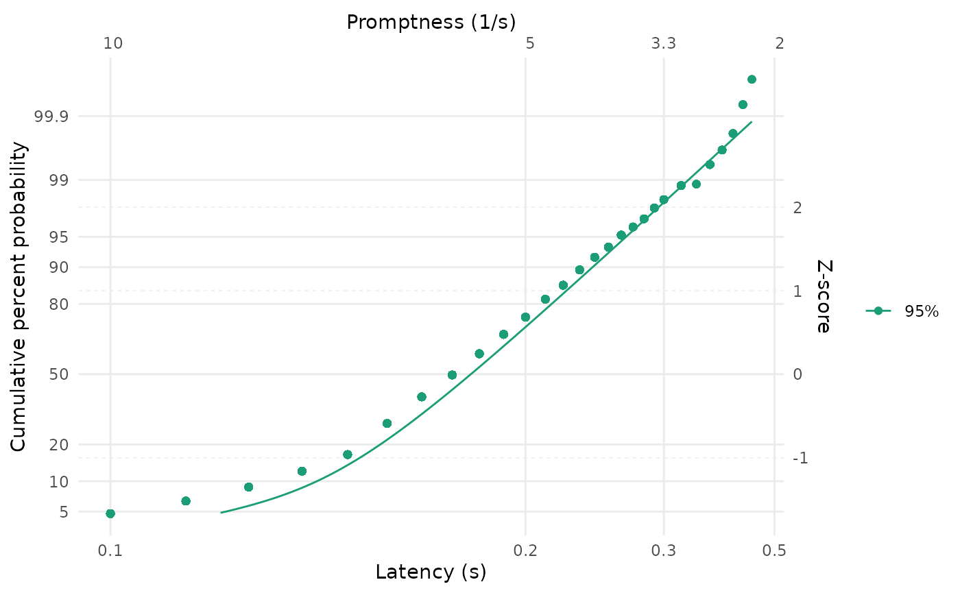
To visually assess the reasonableness of the fitted parameters, we can visualise the fit by passing the variable containing the parameters to the LATERmodel::reciprobit_plot function:

LATERmodel::reciprobit_plot(
  plot_data = data_p95,
  fit_params = fit_p95$named_fit_params
)

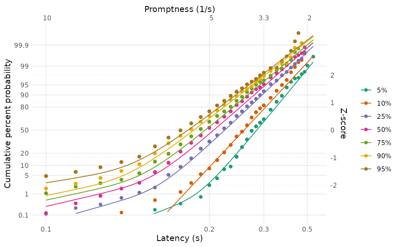
Multiple datasets fitted separately

If we want to fit multiple datasets but consider each dataset separately in the fitting, we can use the LATERmodel::individual_later_fit helper function. Here, we will use it to fit all the conditions in the example data:

individual_named_fit_params <- LATERmodel::individual_later_fit(
  df = data,
  with_early_component = TRUE,
  jitter_settings = list(seed = 561866110)
)

This function returns a dataframe that contains columns for each of the entries in the named_fit_params component of the fit information (along with additional columns relating to the fit):

individual_named_fit_params

name	a	sigma	sigma_e	mu	k	s	fit_criterion	stat	loglike	aic
5%	3.530525	0.6569439	0.7597136	3.530525	5.374164	1.5222000	likelihood	528.2707	-528.2707	1062.541
10%	3.843987	0.6954253	2.4193170	3.843987	5.527534	1.4379690	likelihood	811.0385	-811.0385	1628.077
25%	4.428222	0.8734555	2.9400614	4.428222	5.069775	1.1448781	likelihood	1162.8834	-1162.8834	2331.767
50%	4.843071	0.9573051	3.2493339	4.843071	5.059067	1.0445990	likelihood	2226.8256	-2226.8256	4459.651
75%	5.017060	0.9905442	3.9748709	5.017060	5.064953	1.0095460	likelihood	4110.5947	-4110.5947	8227.189
90%	5.298192	1.0832124	4.2747846	5.298192	4.891185	0.9231800	likelihood	10755.6638	-10755.6638	21517.328
95%	5.438931	1.0911414	5.1809469	5.438931	4.984625	0.9164715	likelihood	17006.1876	-17006.1876	34018.375

We can plot the result, as before.

LATERmodel::reciprobit_plot(
  plot_data = data,
  fit_params = individual_named_fit_params
)

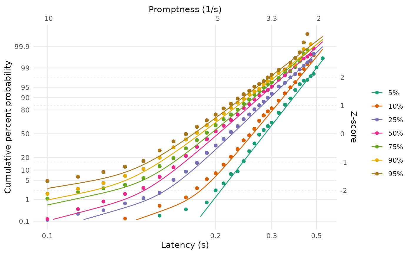
Note that, in contrast to the figure from Carpenter and Williams (1995) shown at the beginning of this document, our plots show the fits from the complete model rather than attempting to isolate the early and primary components. In the following explanation from Carpenter and Noorani (2023), p. 26, about these different plotting approaches, the approach in this package corresponds to the ‘alternative’ that they describe (and their ‘main’ and ‘maverick’ components correspond to our ‘primary’ and ‘early’ components):

“it is important to point out that although for clarity it can often be helpful to plot the asymptotes – in effect, the two separate components corresponding to the main and maverick components – the data points will not be expected to go through them: an alternative is to plot the combined theoretical distribution resulting from both components together”

Multiple datasets fitted together

We might be interested in situations in which multiple datasets have the same LATER model parameter value. We refer to such a scenario as a sharing of model parameters.

Note that it can take a long time for the command to fit a complex LATER model with multiple dataset and shared parameters to complete.

For example, multiple datasets might be considered to have the same scale of the primary component (\(\sigma\)) but vary in the location of the primary component (\(\mu\)) and the scale of the early component (\(\sigma_e\)). This particular arrangement is known as a shift.

To fit the datasets under such a sharing constraint, we use the parameters to the LATERmodel::fit_data function that begin with share_. To implement a shift, we would set share_sigma = TRUE:

fit_shift <- LATERmodel::fit_data(
  data = data,
  with_early_component = TRUE,
  share_sigma = TRUE,
  jitter_settings = list(seed = 268918378)
)

After fitting a LATER model, it is good practice to check that the parameter optimisation algorithm has not reported any issues in producing parameter estimates. This information is contained in the optim_result element within the value returned by LATERmodel::fit_data; in particular, the convergence value (where a nonzero value indicates completion problems; see the documentation for optim) and the message value (which elaborates on any nonzero convergence codes).

fit_shift$optim_result
#> $par
#>  [1] 3.51722099 3.84594345 4.50825807 4.86023422 5.03184333 5.26985858
#>  [7] 5.41248626 0.02299348 0.70937105 0.76752942 0.94380353 1.13359309
#> [13] 1.36615244 1.45198409 1.63118393
#> 
#> $value
#> [1] 36805.59
#> 
#> $counts
#> function gradient 
#>     2988       NA 
#> 
#> $convergence
#> [1] 0
#> 
#> $message
#> NULL

When we look at the fitted parameter values, we can see that they each have the same sigma (and \(s\), which is just \(1 / \sigma\)) - as expected by our request that the \(\sigma\) parameter be shared across datasets:

fit_shift$named_fit_params

	a	sigma	sigma_e	mu	k	s
5%	3.517221	1.02326	2.079993	3.517221	3.437270	0.9772689
10%	3.845944	1.02326	2.204549	3.845944	3.758521	0.9772689
25%	4.508258	1.02326	2.629509	4.508258	4.405780	0.9772689
50%	4.860234	1.02326	3.179063	4.860234	4.749756	0.9772689
75%	5.031843	1.02326	4.011423	5.031843	4.917464	0.9772689
90%	5.269859	1.02326	4.370938	5.269859	5.150069	0.9772689
95%	5.412486	1.02326	5.228777	5.412486	5.289454	0.9772689

We can once again visualise the fits:

LATERmodel::reciprobit_plot(
  plot_data = data,
  fit_params = fit_shift$named_fit_params
)

We can also consider other sharing arrangements. A particularly useful arrangement is known as a swivel, and occurs when multiple datasets share the intercept parameter (\(k\)) in the model. As described in the previous explanation of the model parameters (when fitting a single dataset), the intercept captures the point in z-score space where the response time latency approaches infinity. When sharing the intercept, multiple datasets have the flexibility to rotate or ‘swivel’ around this intercept point.

To be able to share the intercept, we need to tell LATERmodel::fit_data that we would like the \(a\) parameter in the model to refer to \(k\) rather than \(\mu\). We do that by setting the intercept_form parameter to LATERmodel::fit_data to TRUE. We also indicate that we would like this parameter to be shared by setting the share_a parameter to LATERmodel::fit_data to TRUE.

fit_swivel <- LATERmodel::fit_data(
  data = data,
  with_early_component = TRUE,
  intercept_form = TRUE,
  share_a = TRUE,
  jitter_settings = list(seed = 268918378)
)

Note that we have used the same seed for the random jitter as when we fit the ‘shift’ model - this ensures that both models are being compared from the same starting points.

Again, we can check the optimisation convergence:

fit_swivel$optim_result
#> $par
#>  [1]  4.987547312 -0.354059638 -0.236673914 -0.113631820 -0.048725096
#>  [6]  0.001541761  0.065959877  0.085843675  1.142589939  0.267662117
#> [11]  1.211808863  1.330376281  1.366441790  1.371005898  1.565925869
#> 
#> $value
#> [1] 36629.11
#> 
#> $counts
#> function gradient 
#>     3328       NA 
#> 
#> $convergence
#> [1] 0
#> 
#> $message
#> NULL

And we can inspect the fitted parameters:

fit_swivel$named_fit_params

	a	sigma	sigma_e	mu	k	s
5%	4.987547	0.7018331	2.200160	3.500426	4.987547	1.4248402
10%	4.987547	0.7892486	1.031473	3.936415	4.987547	1.2670279
25%	4.987547	0.8925865	2.998695	4.451817	4.987547	1.1203396
50%	4.987547	0.9524429	3.602583	4.750354	4.987547	1.0499317
75%	4.987547	1.0015430	3.927423	4.995243	4.987547	0.9984594
90%	4.987547	1.0681839	4.207909	5.327617	4.987547	0.9361684
95%	4.987547	1.0896360	5.216202	5.434611	4.987547	0.9177377

We can also again plot the fits. Note how the fits are constrained such that they would each meet at a common point on the vertical axis if extrapolated to an infinite latency - this is the consequence of sharing the intercept parameter in the model.

LATERmodel::reciprobit_plot(
  plot_data = data,
  fit_params = fit_swivel$named_fit_params
)

Comparing ‘shift’ and ‘swivel’ fits

We have seen how we can implement different sharing arrangements when fitting multiple datasets. To quantify and compare how well the different sharing arrangements fit the data, we can use the LATERmodel::compare_fits function. This function accepts a named list of variables returned from LATERmodel::fit_data, so we will first construct this variable using the fits for ‘shift’ and ‘swivel’:

fits <- list(shift = fit_shift, swivel = fit_swivel)

We then pass this variable as the argument to the fits parameter in the LATERmodel::compare_fits function:

LATERmodel::compare_fits(fits = fits)

	aic	preferred_rel_fit_delta_aic	preferred_rel_fit_evidence_ratio	preferred
swivel	73288.22	0.0000	1.000000e+00	TRUE
shift	73641.18	-352.9616	4.412071e+76	FALSE

The output from this function contains a row for each of the provided fit results, ordered such that the first row contains the ‘best’ (‘preferred’) fit. This assessment of which fit is ‘best’ is based on the relative Akaike Information Criterion (AIC) values for the fits, where lower AIC values are interpreted as indicating a superior fit in comparison to higher AIC values. The aic column in the table reports these AIC values, and the preferred_rel_fit_delta_aic reports the difference in AIC values between the preferred fit and the AIC value for the fit in the relevant row. In this example, the ‘swivel’ fit is the preferred fit (also indicated in the preferred column) because the ‘swivel’ fit has an AIC that is lower than the AIC for the ‘shift’ fit. Finally, this comparison is also reported as an ‘evidence ratio’ in the preferred_rel_fit_evidence_ratio column. As described in Motulsky and Christopoulos (2004), this evidence ratio “tells you the relative likelihood, given your experimental design, of the two models being correct” (p. 147). Here, the evidence ratio reported in the ‘shift’ row is overwhelmingly high, which indicates that the preferred fit (the ‘swivel’) is much more likely to be the ‘correct’ fit than the ‘shift’ (noting that the evidence ratio is calculated as the ratio of the preferred fit to the fit reported in the row).

Summary

In this walkthrough, we have seen how we can use this package to conduct an analysis of response time data using the LATER model. First, we represented the raw data as a data table having columns for name, condition, and time and having rows corresponding to single trials. We then used the LATERmodel::prepare_data function to convert this raw data into a format suitable for subsequent analysis. We used the LATERmodel::fit_data function to fit the parameters of a LATER model to such data; either for a single dataset, multiple datasets considered separately, or multiple datasets with sharing of LATER model parameters. We saw how we could use the LATERmodel::reciprobit_plot to visualise both the observed data and model fits in the ‘reciprobit’ space used in the LATER model. Finally, we used the LATERmodel::compare_fits function to compare the goodness-of-fit of multiple fits to data.

References

Carpenter, R. H. S., and Imran Noorani. 2023. LATER: The Neurophysiology of Decision-Making. Cambridge, United Kingdom: Cambridge University Press. https://doi.org/10.1017/9781108920803.

Carpenter, R. H. S., and M. L. L. Williams. 1995. “Neural Computation of Log Likelihood in Control of Saccadic Eye Movements.” Nature 377 (6544): 59–62. https://doi.org/10.1038/377059a0.

Motulsky, Harvey, and Arthur Christopoulos. 2004. Fitting Models to Biological Data Using Linear and Nonlinear Regression: A Practical Guide to Curve Fitting. Oxford University PressNew York, NY. https://doi.org/10.1093/oso/9780195171792.001.0001.