Model fitting

Here, we will look at an example of fitting a model to an example dataset.

First, we will import the necessary packages:

import pymc as pm

import pylater
import pylater.data

We will use the 50% condition from participant ‘a’ in the example data provided in pylater:

dataset = pylater.data.cw1995["b_p50"]

We can then build the model, using the default priors, via:

model = pylater.build_default_model(datasets=[dataset])

We can then fit the model by using the sample function from PyMC:

with model:
    idata = pm.sample(chains=4)

We can then use the posterior summary methods from PyMC to evaluate the posteriors:

pm.stats.summary(data=idata)

	mean	sd	hdi_3%	hdi_97%	mcse_mean	mcse_sd	ess_bulk	ess_tail	r_hat
k[b_p50]	5.063	0.107	4.860	5.264	0.003	0.002	1418.0	1455.0	1.0
mu[b_p50]	4.842	0.029	4.786	4.894	0.000	0.000	3506.0	3051.0	1.0
sigma[b_p50]	0.957	0.020	0.919	0.996	0.001	0.000	1359.0	1299.0	1.0
sigma_e[b_p50]	3.256	0.132	2.998	3.495	0.003	0.002	1749.0	1784.0	1.0
sigma_e_mod[b_p50]	3.405	0.171	3.096	3.738	0.005	0.003	1357.0	1153.0	1.0

We can futher evaluate the model fit by examining the distribution of draws from the fitted model - the posterior predictive distribution (better described as the posterior retrodictive distribution; see “Towards a principled Bayesian workflow” by Michael Betancourt):

First, we need to use PyMC to sample the posterior predictives:

with model:
    idata = pm.sample_posterior_predictive(trace=idata, extend_inferencedata=True)

We can then use the plot_predictive method of a ReciprobitPlot instance to visualise the posterior predictives:

plot = pylater.ReciprobitPlot()
plot.plot_predictive(idata=idata, predictive_type="posterior");

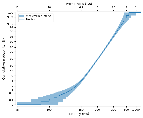
In the above, we can see the 95% credible interval and median of the distribution of posterior predictive samples.

This becomes particularly useful when compared against the ECDF of the observed data:

plot = pylater.ReciprobitPlot()
plot.plot_predictive(idata=idata, predictive_type="posterior");
plot.plot_data(data=dataset);

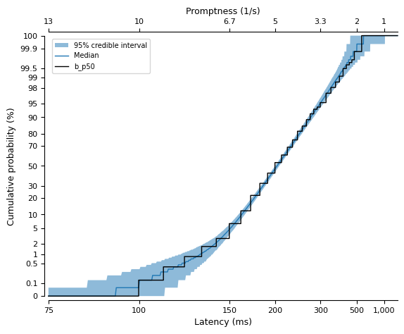
We can see a reasonably good correspondence between the observations and the draws from the fitted model.

Last updated: Wed May 15 2024

Python implementation: CPython
Python version       : 3.10.14
IPython version      : 8.24.0

matplotlib: 3.8.4

pylater: 0.1
pymc   : 5.15.0