Prior distributions

Performing Bayesian analysis requires careful consideration of the prior distributions for the model parameters. Here, we will consider how priors are treated in pylater and look at a method for visualising the influence of the priors.

First, we will import the necessary packages:

import pymc as pm

import pylater
import pylater.data

Default priors

pylater uses the PyMC package for describing LATER models and is intended for use by practitioners familiar with PyMC (or willing to become familiar with PyMC). However, pylater also provides the function build_default_model that assembles a PyMC model for given data using a default set of priors. This function is intended to provide an example of how LATER model priors can be specified, and should not be used without assessing the priors that it uses.

We will examine the usage of build_default_model using some example data:

dataset = pylater.data.cw1995["b_p50"]

We can then build the model, using the default priors, via:

model = pylater.build_default_model(datasets=[dataset])

Plotting the effect of priors

We can visualise the prior distributions for parameters using the ArviZ package. However, it is particularly useful to look at the distribution of reaction times that is produced by the priors - the prior predictive distribution.

First, we need to sample the prior predictives using PyMC:

with model:
    idata = pm.sample_prior_predictive()

We then use the plot_predictive method of a reciprobit plot variable:

plot = pylater.ReciprobitPlot()
plot.plot_predictive(idata=idata, predictive_type="prior");

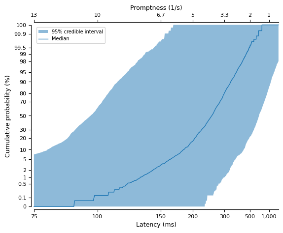
This shows the 95% credible range and the median of the ECDFs that would be expected to be encountered given our (default) priors.

Last updated: Wed May 15 2024

Python implementation: CPython
Python version       : 3.10.14
IPython version      : 8.24.0

matplotlib: 3.8.4

pymc   : 5.15.0
pylater: 0.1