Cheat sheet

A quick overview of crategraph's basics: loading a crate, exploring its entities and relationships, filtering and transforming the graph, and visualising the result.

Open the cheat sheet as a PDF

Inspired by Franz Diebold's Polars cheat sheet.

The data model

A crate loaded with crategraph is a Graph with two layers: entities (the nodes: people, files, places, events), and relationships (the directed edges that link them).

graph LR
    A("<b>Entity</b> (node)<br/>id · types · name · properties")
    B("<b>Entity</b> (node)<br/>id · types · name · properties")
    A -->|"<b>Relationship</b> (edge)<br/>type · source · target · properties"| B

Each layer has its own accessor and its own filter:

Layer	What it holds	List them	Filter by
Entities (nodes)	id, types, name, properties	crate.entities	where() - a property value
Relationships (edges)	type, source, target, properties	crate.relationships	select() - a type or structure

The queried layer must match the method. For example, crate.where(relationship_types="Primary") returns 0 results: where looks for a node property literally named relationship_types, which does not exist; matching a relationship type is select's job (crate.select(relationship_types="Primary" will return results)).

Every filter/transformation returns a new Graph, so they chain.

Load a graph

We explore the package on the University of Melbourne Perpetual Calendar (UMPC) crate, from the OHRM Upload Project. Source: umpc.esrc.unimelb.edu.au.

Load a crate (RO-Crate) from a local directory containing ro-crate-metadata.json:

from crategraph import Crate

crate = Crate("data/ohrm/UMPC")
crate

Graph(4270 entities, 12601 relationships, source='data/ohrm/UMPC')

A few load-time options:

Crate(p1, p2)                       # load several crates (IDs prefixed by directory name)
Crate(path, include_root=True)      # keep the root Dataset entity as a node
Crate(path, inline_relations=False) # only reified Relationship entities become edges

Get a feel for the crate

A summary of the graph, including the full list of entity types and relationship counts:

crate.summary()

=== Graph Summary ===
Source: data/ohrm/UMPC
Entities: 4270 | Relationships: 12601

Entity types:
  PublishedResource, Resource                  1068  ▒▒▒▒▒▒▒▒▒▒▒▒▒▒▒
  Regulations_and Statutes                      751  ▒▒▒▒▒▒▒▒▒▒▒
  Person                                        554  ▒▒▒▒▒▒▒▒
  Person, University of Melbourne               317  ▒▒▒▒
  Role                                          200  ▒▒▒
  ...

Structural stats: density, components, connectivity and the connection distribution:

crate.profile()

=== Graph Profile ===
Source: data/ohrm/UMPC
Entities: 4270 | Relationships: 12601
Density: 0.0007
Types: 54 entity, 17 relationship

Entity types:
  PublishedResource         1343  ▒▒▒▒▒▒▒▒▒▒▒▒▒▒▒
  Person                     907  ▒▒▒▒▒▒▒▒▒▒
  Regulations_and Statutes   751  ▒▒▒▒▒▒▒▒
  ...

Relationship coverage across entity types (useful for spotting data-quality gaps in the RO-Crate metadata):

crate.coverage()

[CoverageResult(Related source: 6/907 Person (1%)),
 CoverageResult(Related target: 6/907 Person (1%)),
 ...
 CoverageResult(Related source: 42/42 Individual_Story (100%))]

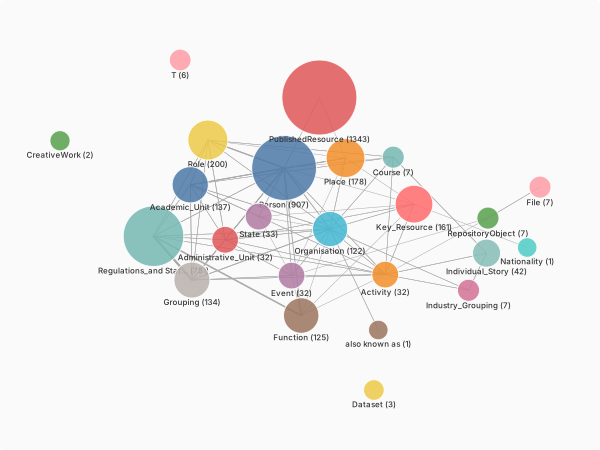
A visual snapshot of the graph (collapsed to a type-level overview):

crate.glimpse()

Entities (nodes)

Each item in a crate (people, files, places) has .properties (a data dictionary) and a .types attribute.

Look around: what does this graph contain?

crate.entities          # list[EntityView] of all nodes

Explore a single entity. Index the list (crate.entities[0]), or find a specific one (filter by an exact property):

e = crate.where(name="UTR7.166 The Olga Lawless Ziegler Memorial Fund").entities[0]
e

EntityView('Regulations_and Statutes', 'UTR7.166 The Olga Lawless Ziegler Memorial Fund', id='#E001213')

Get all file entities:

crate.files

A sorted list of all entity type names present in the graph:

list(crate.types)

['Academic_Unit', 'Activity', 'Administrative_Unit', 'Article', 'Book', 'BookSection', ...]

The number of entities (also visible in .profile()):

len(crate)

4270

Inspecting an individual entity

print(e)

EntityView('Regulations_and Statutes', 'UTR7.166 The Olga Lawless Ziegler Memorial Fund', id='#E001213')

Most of what you need is in .properties:

e.properties

{'identifier': 'E001213',
 'name': 'UTR7.166 The Olga Lawless Ziegler Memorial Fund',
 'function': 'Scholarship',
 'processingNotes': '16 October 2018 Alannah Croom. Created entity',
 ...}

Properties are read-only

properties is a read-only view — in-place mutation raises TypeError. Derive new fields with annotate_entities(...) instead.

Get a specific entity by id. Like every accessor, this returns a graph-aware EntityView, so you can traverse straight from it:

crate.get(e.id)

If anything is unclear, call help() on an object:

help(e)

List all property keys

To see which property keys appear across the graph:

sorted({k for e in crate.entities for k in e.properties})

Count distinct property values:

Return a count of distinct values for any property, sorted by count, descending:

crate.entity_counts("function")

[{'function': 'Scholarship', 'count': 259},
 {'function': 'Research Fund', 'count': 57},
 {'function': 'Prize', 'count': 36},
 ...
 {'function': 'Lawyer', 'count': 13}, ...]

crate.entity_counts("type")

[{'type': 'PublishedResource', 'count': 1343},
 {'type': 'Person', 'count': 907},
 {'type': 'Regulations_and Statutes', 'count': 751},
 ...]

Entities as records

entity_records() returns one dictionary per entity (id, label, type, then its properties), ready to hand to pandas or polars for a DataFrame, or to write out. Pass columns to keep only the fields you need:

crate.entity_records(columns=["id", "label", "type"])

[{'id': 'ro-crate-metadata.json', 'label': 'ro-crate-metadata.json', 'type': 'CreativeWork'},
 {'id': '#D00000001', 'label': 'The Scholarly, Teaching, Research and Engagement History of The University of Melbourne', 'type': 'RepositoryObject'},
 ...]

See From Graph to DataFrame for the full tabular workflow.

Filter entities by property

Find all the lawyers in the graph:

crate.where(function="Lawyer")

Graph(13 entities, 0 relationships, source='data/ohrm/UMPC')

Find all the entries within a date period (inclusive):

crate.where(startDate=(1870, 1900))

Graph(70 entities, 130 relationships, source='data/ohrm/UMPC')

Enrich entities with derived properties

If we want to see people born in Victoria, we start by finding out what Victoria is linked to:

crate.annotate_entities(
    place=lambda e: e.related("birthPlace").first("name")
).entity_counts("place")

[{'place': 'Melbourne', 'count': 19},
 {'place': 'University of Melbourne', 'count': 8},
 {'place': 'Sydney', 'count': 6}, ...]

crate.annotate_entities(
    state=lambda e: e.related("birthState").first("name")
).entity_counts("state")

[{'state': 'Victoria', 'count': 98},
 {'state': 'New South Wales', 'count': 12}, ...]

Now that we know Victoria is the value of a birthState, we can add a new property to entities and filter on it:

crate2 = crate.annotate_entities(
    is_victorian=lambda e: e.related("birthState").first("name") == "Victoria"
)
len(crate2.where(is_victorian=True))

98

Find the top hub entities in the graph (10 by default, adjust the amount of connections n if needed):

crate.most_connected(n=3)

[(EntityView('Regulations_and Statutes', 'Chapter R6, Prizes, Exhibitions, Scholarships and Bursaries', id='#E000100'), 417),
 (EntityView('Function', 'Scholarship', id='#F000001'), 331),
 (EntityView('Regulations_and Statutes', 'Chapter R7, Endowments Other Than Those of Prizes, Exhibitions and Scholarships', id='#E001373'), 321)]

Relationships (edges)

Directed links between entities. Each has a .type, .source and .target.

Look at what relationship types exist in the graph:

list(crate.relationship_types)

['Previous', 'Primary', 'Related', 'Relationship', 'Subsequent', 'alsoKnownAs',
 'birthPlace', 'birthState', 'deathPlace', 'deathState', 'dobject', 'entity',
 'hasFile', 'nationality', 'place', 'preparedBy', 'relatedEvents']

Inspect a single relationship object:

print(crate.relationships[111])

Relationship('#E000018' --deathState--> '#Victoria')

Count relationships by type

A count of how many relationships exist for each type, sorted by count (descending):

crate.relationship_counts("type")

[{'type': 'Related', 'count': 9743},
 {'type': 'Relationship', 'count': 1249},
 {'type': 'entity', 'count': 358}, ...]

relationship_records() is the edge counterpart of entity_records(): one dictionary per edge, ready for a DataFrame or export.

crate.relationship_records(columns=["source", "target", "type"])

[{'source': '#D00000001', 'target': 'objects/documents/Appendix 1_2017-03-20 Proposal for VC.pdf', 'type': 'hasFile'},
 ...]

Filter by relationship type (select)

Find entities connected by a Primary relationship:

crate.select(relationship_types="Primary")

Graph(10 entities, 15 relationships, source='data/ohrm/UMPC')

You can match several relationship types at once:

crate.select(relationship_types=["Previous", "Related"])

Graph(2206 entities, 9767 relationships, source='data/ohrm/UMPC')

pattern() matches by the relationship type on the edge. Everything connected via a preparedBy edge (source or target):

crate.pattern(via="preparedBy")

Graph(266 entities, 561 relationships, source='data/ohrm/UMPC')

Enrich relationships with derived properties

annotate_relationships() derives a property per edge from a function that receives a RelationshipView (with .source, .target, .type). For example, label each edge with the entity types it connects, then count the type-to-type pairs:

typed = crate.annotate_relationships(
    pair=lambda r: f"{r.source.types[0]} -> {r.target.types[0]}"
)
typed.relationship_counts("pair")

[{'pair': 'Regulations_and Statutes -> Regulations_and Statutes', 'count': 1507},
 {'pair': 'Grouping -> Regulations_and Statutes', 'count': 1170},
 {'pair': 'Person -> Person', 'count': 721}, ...]

collapse_edges() merges parallel edges between the same pair of nodes into single summary edges, a quick way to thin a dense graph:

collapsed = crate.collapse_edges()
len(crate.relationships), len(collapsed.relationships)

(12601, 7307)

File content

The data files attached to file-entities:

len(crate.files)

10

The UMPC files are document records without extracted text, so the text features below are shown as syntax; see the linked tutorials for crates that carry file text.

text_records() pulls the text out of file entities (one record per file), with each file's entity metadata attached, ready for NLP. It returns an iterator, so step through it with next(...) or collect it with list(...):

record = next(crate.text_records(include_properties=["name"]))
record["entity_id"], record["text"][:200]

See Basic NLP with Text Records for a worked example.

Search file text by meaning (semantic)

Fuzzy search() (in the Graph manipulations card) matches the metadata; semantic search reads the file text. Build a semantic index once (this needs the [index] extra and downloads a small embedding model), then query it. The index persists at store_path and is reused by later searches:

crate.build_semantic_index(store_path="crate-index.db")
crate.search("scholarships for women", mode="semantic", store_path="crate-index.db")

chunk_records() returns the ranked passages behind a semantic search, with scores, for a results-list view:

next(crate.chunk_records("scholarships for women", store_path="crate-index.db", k=1))

See Searching a Collection for the full semantic-search walk-through.

Graph manipulations

Each manipulation returns a new graph.

Filter and subset

Select a single entity type:

people = crate.select(entity_types=["Person"])

Graph(907 entities, 721 relationships, source='data/ohrm/UMPC')

A time period:

mid_cent = crate.select(time_range=(1945, 1960))

Graph(268 entities, 346 relationships, source='data/ohrm/UMPC')

The most connected entities:

crate.select(min_connections=20)

Graph(79 entities, 128 relationships, source='data/ohrm/UMPC')

You can also leave information out. Exclude a relationship type:

crate.exclude(relationship_types="Related")

Graph(3274 entities, 2858 relationships, source='data/ohrm/UMPC')

drop() removes the entities whose given property contains a value. Here we drop everything prepared by the most prolific preparer, found from the data itself:

preparer = crate.entity_counts("preparedBy")[0]["preparedBy"]   # '#Alannah Croom'
crate.drop(preparer, property="preparedBy")

Graph(4122 entities, 11466 relationships, source='data/ohrm/UMPC')

drop() returns 4122 entities, while the opposite where() returns 148. Together they make up the original 4270:

prepared = crate.where(preparedBy=preparer)
prepared

Graph(148 entities, 300 relationships, source='data/ohrm/UMPC')

Take the entities of one graph out of another with subtract():

crate.subtract(prepared)

Graph(4122 entities, 11466 relationships, source='data/ohrm/UMPC')

Free-text search for an entity. The default minimum rapidfuzz match score is 80; both the threshold and the number of results are adjustable:

crate.search("Elisabet")

Graph(120 entities, 73 relationships, source='data/ohrm/UMPC')

crate.search("Elisabeth", threshold=90, top_n=3)

Graph(8 entities, 0 relationships, source='data/ohrm/UMPC')

Transform: dates, merging, communities

Raw string dates (like "1985", "c.1920s", or "1 March 2003") can be parsed into ISO date columns:

crate.convert_dates()

convert_dates: parsed 1643/1643 entities with date fields (100%).

… or you can specify the fields to convert:

crate.convert_dates(start="startDate", end="endDate")

merge_nodes() aggregates nodes by a property, returning a collapsed graph. Merging by type gives a compact, type-level view: one node per type, each carrying a count, and weighted type-to-type edges.

overview = crate.merge_nodes(by="type")
overview

Graph(47 entities, 177 relationships, source='data/ohrm/UMPC')

overview.get("Person").properties

{'label': 'Person', 'count': 554, 'merged_by': 'type'}

Add a community property to the graph with the Louvain algorithm (pass a seed for a reproducible result):

communities = crate.detect_communities(seed=42)
communities.entity_counts("community")

[{'community': 23, 'count': 772},
 {'community': 5, 'count': 470},
 {'community': 18, 'count': 344}, ...]

Then isolate the largest community:

communities.where(community=23)

Graph(772 entities, 2687 relationships, source='data/ohrm/UMPC')

expand() grows a selection outward to include connected neighbours. Start from the 13 lawyers and pull in everything one layer away:

lawyers = crate.where(function="Lawyer")   # 13 entities
lawyers.expand(depth=1)                      # 62 entities

query() matches a Cypher-style pattern and returns the matched subgraph. For example, people with a recorded birthplace:

crate.query("(a:Person)-[:birthPlace]->(b:Place)")

Graph(263 entities, ...)

Visualising and exporting

The default renderer for visualise() is "2d" (sigma.js, WebGL). Other options are "3d" (3d-force-graph), "svg" (static SVG) and "pyvis" (vis.js, requires an additional install).

crate.visualise(colour_by="type", filepath="umpc-network.html")

The same call takes a renderer and styling options. These write standalone HTML files you can open in a browser:

crate.visualise(renderer="3d", filepath="umpc-3d.html")
crate.visualise(colour_by="community", size_by="year", filepath="umpc-styled.html")

For crates with images, gallery() lays the image-bearing entities out as a thumbnail grid (UMPC holds documents rather than images, so see Building a Thumbnail Gallery for a worked example):

crate.gallery(columns=4, filepath="gallery.html")

Export GraphML to open the crate in Gephi or Cytoscape:

crate.write("crate_export.graphml", format="graphml")

... or hand the graph to NetworkX to use its algorithms directly:

crate.to_networkx()    # -> NetworkX MultiDiGraph with 4270 nodes and 12601 edges