Mapping the places in a collection
Many RO-Crates record where something happened, but the geography rarely sits
where you might expect. A place's coordinates are usually not on the place itself;
they hang off a separate geometry entity, written as a line of
Well-Known Text
(WKT) such as POINT(151.21 -33.86) or a POLYGON(...). This tutorial walks from a
loaded crate to an interactive map, following those links, reading the coordinates
out of the WKT, and finishing with several collections side by side, coloured by
the crate each place came from.
We'll use the Farms to Freeways example dataset from the Language Data Commons of Australia (LDACA), an oral-history collection about the suburbanisation of western Sydney. Its records are anchored to the street addresses where interviews were recorded.
What you'll learn
- Finding the
Placeentities in a crate and the geometry linked to each one. - Reading coordinates out of WKT, for both points and polygons, with shapely.
- Annotating places with
longitude/latitudecolumns and flattening to pandas. - Drawing an interactive map with Plotly Express.
- Putting several crates on one map, coloured by their origin.
- Geocoding place names when a crate records no coordinates at all.
Running this tutorial
Install crategraph with Jupyter and the plotting and geocoding dependencies, then launch a notebook:
1. Load the crate and find the places
from crategraph import Crate

crate = Crate("data/ldaca/metadata_only/Farms_to_Freeways_Example_Dataset")
crate
Graph(763 entities, 1765 relationships, source='data/ldaca/metadata_only/Farms_to_Freeways_Example_Dataset')
Before zooming in, glimpse() gives a one-look overview. It collapses every entity to its
primary type, so you can see what kinds of thing the crate holds and how they connect, a handy
orientation before committing to a query (in a notebook it renders inline):
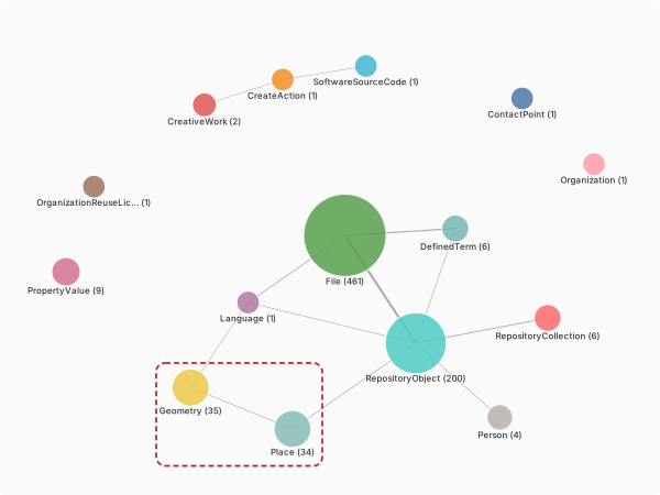
Each node is an entity type, labelled with its count; the lines are relationships between
those types. Most of the crate is the interviews and their media, File (461) and
RepositoryObject (200), but the two types carrying the geography are boxed in red:
Place (34) and Geometry (35), joined by a single edge. That link is the whole story
of this tutorial: a place does not hold its own coordinates, it points to a separate
Geometry that does. We follow that edge below.
select() narrows the graph to a single type. The locations are Place entities:
Graph(34 entities, 0 relationships, source='data/ldaca/metadata_only/Farms_to_Freeways_Example_Dataset')
Thirty-four places, and notice the 0 relationships: narrowing to Place has dropped
every edge, because the entities those edges pointed to are not themselves places. That
matters in a moment, because the coordinates live on the other end of one of those edges.
2. Follow a place to its geometry
Pick one place and look at its raw properties:
{'address': '131 Macquarie st, sydney',
 '@label': '131 Macquarie st, sydney',
 'geo': 'http://omeka.uws.edu.au/farmstofreeways/api/geolocations/24#GEO'}
There is a human-readable address, but no latitude or longitude. The geo property is
not a coordinate; it is a reference to a separate Geometry entity. Those geometry
entities are where the coordinates live, written as Well-Known Text. We can look at one
directly:
That asWKT value is a coordinate written as Well-Known Text, the form the
RO-Crate guidance recommends
for a Place's geometry (a place should reference a Geometry entity whose asWKT
expresses the point or shape in WKT). POINT(lon lat) lists longitude first, then
latitude, which is western Sydney. Two wrinkles show up across crates: some store the WKT
directly on the Place (no geo hop), and some namespace the key as geo:asWKT rather
than asWKT. The helper in the next step handles all three cases, linking each place to its
own geometry.
3. From WKT to coordinates
We don't have to parse WKT by hand; shapely reads it.
wkt.loads turns the string into a geometry object, and .centroid collapses any shape to a
single point: a POINT returns itself, while a POLYGON (a postcode or a state boundary)
returns its centre. That keeps every place, whatever the shape of its geometry, to one
mappable point:
from shapely import wkt

shape = wkt.loads(
    "POLYGON((140.999271 -37.505041, 153.638673 -37.505041, "
    "153.638673 -28.157015, 140.999271 -28.157015, 140.999271 -37.505041))"
)
shape.centroid.x, shape.centroid.y
A small helper finds a place's WKT (on the entity itself or on a linked geometry, under
either key) and hands it to shapely. Here e is an entity view, the object an
annotate_entities function receives, which is what lets it follow the geo link:
def place_point(e):
    """A place's geometry as a shapely point (its own POINT or a POLYGON's centroid),
    whether the WKT sits on the place itself or on a linked Geometry."""
    raw = (e.get("asWKT") or e.get("geo:asWKT")
           or e.related("geo").first(key="asWKT")
           or e.related("geo").first(key="geo:asWKT"))
    if not raw:
        return None
    return wkt.loads(raw[0] if isinstance(raw, list) else raw).centroid
We put it to work in the next step.
4. Build a table of mapped places
annotate_entities adds a field to every entity, computed by a small function we supply
(the lambda e: ... is a one-line function in which e is one entity). Because the
coordinates are reached through the geo edge, we annotate the whole crate (where that
edge exists) and only then narrow to the places:
import pandas as pd

located = crate.annotate_entities(
    longitude=lambda e: place_point(e).x if place_point(e) else None,
    latitude=lambda e: place_point(e).y if place_point(e) else None,
).select(entity_types=["Place"])

df = pd.DataFrame(located.entity_records(columns=["address", "longitude", "latitude"]))
df = df.dropna(subset=["latitude"])
print(len(df), "places with coordinates")
df.head()
                    address  longitude   latitude
  74 River Road, Emu Plains 150.666511 -33.756987
                            150.708486 -33.754658
36 Lalor Road, Quakers Hill 150.889739 -33.727179
                            150.661456 -33.760737
  4 Colless Street, Penrith 150.708667 -33.756918
All thirty-four places resolved to a coordinate in the western-Sydney corridor: Emu Plains,
Quakers Hill, Penrith. The dropna keeps only the places that have
coordinates; everything else is plain pandas. Two things are worth noticing: the rows arrive
in no particular order (sort them if you want a tidy table, but the map won't care), and a
couple of places carry coordinates without a street address, both fine for plotting.
5. Draw the map
With longitude and latitude columns in hand, Plotly Express puts them on a slippy map.
map_style="open-street-map" uses OpenStreetMap tiles and needs no account or token:
import plotly.express as px

fig = px.scatter_map(
    df, lat="latitude", lon="longitude", hover_name="address",
    center=dict(lat=df["latitude"].mean(), lon=df["longitude"].mean()),
    zoom=10, height=430, map_style="open-street-map",
)
fig.update_traces(marker=dict(size=11, color="#c1272d", opacity=0.8))
fig.update_layout(margin=dict(l=0, r=0, t=0, b=0))
fig.show()
The map below is interactive: scroll to zoom, drag to pan, and hover any marker to read its address. The cluster sits across the western suburbs of Sydney, with a couple of outliers in the city centre.
6. Several collections on one map, coloured by origin
The same pattern works on any crate, so we can compare collections. We wrap the
annotate-then-select from the last section into one function (given a crate path, it returns
the places that have coordinates as plain dicts) and run it over three LDACA corpora.
entity_records already hands back dicts, so combining is just adding an origin key and
appending. Each crate labels its places differently (a street address in one, a postcode or
region name in another), so place_label takes whichever is present. Reducing every geometry
to a centroid means one crate's postcode polygons and another's address points become
comparable markers:
from collections import Counter

def place_label(e):
    """A readable label for a place: its street address, or its name."""
    name = e.name
    if isinstance(name, list):
        name = name[0] if name else None
    return e.get("address") or name

def place_records(path):
    """Load a crate and return its places that carry coordinates, as plain dicts."""
    located = Crate(path).annotate_entities(
        place=place_label,
        longitude=lambda e: place_point(e).x if place_point(e) else None,
        latitude=lambda e: place_point(e).y if place_point(e) else None,
    ).select(entity_types=["Place"])
    return [r for r in located.entity_records(columns=["place", "longitude", "latitude"])
            if r["latitude"] is not None]

sources = {
    "Farms to Freeways": "data/ldaca/metadata_only/Farms_to_Freeways_Example_Dataset",
    "Slang Survey":      "data/ldaca/metadata_only/Australian_Slang_Survey_Data",
    "COOEE":             "data/ldaca/metadata_only/A_COrpus_of_Oz_Early_English__COOEE_",
}

places = []
for origin, path in sources.items():
    for record in place_records(path):
        # COOEE also records England; keep markers within Australia
        if 110 < record["longitude"] < 155 and -45 < record["latitude"] < -9:
            places.append(record | {"origin": origin})

Counter(p["origin"] for p in places)
The three crates carry geography at very different grains: the Slang Survey pins respondents to 1,235 postcode areas, Farms to Freeways to 34 Sydney street addresses, and COOEE to a handful of colony- and state-sized regions. Colouring by origin shows each collection's footprint at a glance:
allplaces = pd.DataFrame(places)   # one DataFrame, only because Plotly wants one

origin_colours = {
    "Farms to Freeways": "#c1272d",   # the same red as the single-crate map above
    "Slang Survey": "#1f77b4",
    "COOEE": "#6a3d9a",               # purple, since green blends into the base map
}

fig = px.scatter_map(
    allplaces, lat="latitude", lon="longitude", color="origin",
    color_discrete_map=origin_colours,
    # draw the populous Slang Survey first, so the rarer crates sit on top
    category_orders={"origin": ["Slang Survey", "Farms to Freeways", "COOEE"]},
    hover_name="place", zoom=3.2, height=480, map_style="open-street-map",
)
fig.update_traces(marker=dict(size=9, opacity=0.7))
fig.update_layout(margin=dict(l=0, r=0, t=0, b=0), legend_title_text="Origin crate")
fig.show()
The Slang Survey blankets the populated south-east, Farms to Freeways concentrates on western Sydney, and COOEE's centroids spread thinly across the colonies. Use the legend to hide a crate and compare the others.
7. When a crate has only place names: geocoding
Not every crate ships coordinates. Many record a location as nothing but a name, and then there is no WKT to read, so you have to geocode: ask a service to turn "Ballarat" or "Naples" into a latitude and longitude. The University of Melbourne (UMPC) crate from the temporal tutorial is one of these; its places are the birthplaces and deathplaces of the people it records.
umpc = Crate("data/ohrm/UMPC-ro-crate")
umpc_places = umpc.select(entity_types=["Place"])
umpc_places.where(name="Balwyn").entities[0].properties
A name and nothing else: no geo link and no asWKT, so place_point would return None
here; there is simply nothing to parse. To map these places we geocode their names.
We'll use geopy, which wraps many geocoding services. Its
free OpenStreetMap geocoder, Nominatim, needs no account, only a descriptive user_agent
and, by its usage policy, no more
than one request per second. RateLimiter enforces that pace for us. Start with one place:
from geopy.geocoders import Nominatim
from geopy.extra.rate_limiter import RateLimiter

geocoder = Nominatim(user_agent="crategraph-mapping-tutorial/1.0")
geocode = RateLimiter(geocoder.geocode, min_delay_seconds=1.5)

location = geocode("Balwyn, Victoria, Australia")
location.address, location.latitude, location.longitude
Geocoding the whole collection
Now scale up to every birthplace. Two habits matter. First, cache: look each name up
once and reuse the answer, so a re-run doesn't hammer the service. Second, be patient:
at roughly one request per second, ~180 places take a few minutes. The to_coords helper
caches into a dict, so the two lookups for latitude and longitude cost only one request:
cache = {}

def to_coords(e):
    if e.name not in cache:
        cache[e.name] = geocode(e.name)
    return cache[e.name]

located = umpc_places.annotate_entities(
    latitude=lambda e: to_coords(e).latitude if to_coords(e) else None,
    longitude=lambda e: to_coords(e).longitude if to_coords(e) else None,
)
gdf = pd.DataFrame(located.entity_records(columns=["name", "latitude", "longitude"]))
gdf = gdf.dropna(subset=["latitude"])
print(f"geocoded {len(gdf)} of {len(umpc_places.entities)} places")
Sixteen names did not resolve, and a few that did landed in the wrong place; geocoding a
bare name is inherently ambiguous. "113 Prospect Rd, Newton" came back in Mississippi,
because "Newton" matches towns the world over. In practice you would add context to the
query (f"{name}, Australia"), inspect the returned location.address before trusting it,
or switch to a paid or self-hosted geocoder for bulk work. For a first map, the resolved
majority is enough:
fig = px.scatter_map(
    gdf, lat="latitude", lon="longitude", hover_name="name",
    zoom=1, height=480, map_style="open-street-map",
)
fig.update_traces(marker=dict(size=9, color="#2a6f97", opacity=0.75))
fig.update_layout(margin=dict(l=0, r=0, t=0, b=0))
fig.show()
The birthplaces cluster in Victoria and around Melbourne, with a strong tail back to Britain and Europe, the shape you would expect of a nineteenth- and twentieth-century Australian university. Hover any marker for the place name.
Next steps
Because annotate_entities writes plain columns, the mapped coordinates feed straight into
the From Graph to DataFrame workflow: group places by region,
write a CSV, or join the geography onto the rest of your analysis. Pair the map with
Exploring Temporal Dimensions to ask not just where a
collection's records sit, but when.