From Graph to DataFrame
This tutorial walks through one common workflow: loading a crate, adding a couple of derived fields to the entities, filtering on one of them, and producing a pandas DataFrame and CSV from the result. We'll use a small example crate of six people across four decades.
What you'll learn
- Getting a quick overview of a crate with
summary(). - Looking at the properties of a single entity to see what's available.
- Adding new fields to entities with
annotate_entities. - Using a derived field anywhere a native property would work, including in
where()filters and invisualise(). - Turning the entities into a pandas DataFrame and writing a CSV.
The example crate is at docs/tutorials/data/people-demo/ in the repository. It has six people with birth dates spanning four decades, two organisations, and some knows connections between the people.
1. Load the crate
2. Get the lay of the land
=== Graph Summary ===
Source: docs/tutorials/data/people-demo
Entities: 8 | Relationships: 12

Entity types:
  Person        6  ▒▒▒▒▒▒▒▒▒▒▒▒▒▒▒
  Organisation  2  ▒▒▒▒▒

Relationship types:
  knows        7  ▒▒▒▒▒▒▒▒▒▒▒▒▒▒▒
  affiliation  5  ▒▒▒▒▒▒▒▒▒▒▒

Most connected: Rita Okafor (5), Amelia Hoxha (4), Elena Marchetti (3), Tom Pereira (3), Heritage Studies Centre (3)
Six people, two organisations, and two kinds of connection: affiliation from a person to their organisation, and knows between people.
3. Look at a person's properties
Before we add any new fields, it helps to see what's already there. Pick any person and look at their properties:
{'name': 'Elena Marchetti', 'birthDate': '1962-03-04', 'affiliation': '#org-heritage', 'knows': ['#person-tom', '#person-rita']}
That gives you a feel for what each person carries. Different people may have slightly different sets of properties. Elena has an affiliation, but not every person does. To see every property name that appears anywhere across the people, collect them as you loop through:
all_names = set()
for person in crate.select(entity_types=["Person"]).entities:
    all_names.update(person.properties)
sorted(all_names)
In the next step we'll add a new field that's the same for everyone.
4. Add a derived field with annotate_entities
birthDate is a string. To group people by decade, sort them chronologically, or compute an age, we want it as a number we can do arithmetic with. crategraph has native temporal accessors that parse date properties for you, so there's no need to pick the string apart by hand. annotate_entities adds a new field to every entity, calculated from a small function we provide:
people = crate.select(entity_types=["Person"]).annotate_entities(
    birth_year=lambda e: e.parse_year("birthDate"),
)
The lambda e: ... part is just Python's compact way of writing a one-line function. It's called once per person; e is the person, and e.parse_year("birthDate") reads their birthDate property and returns the year as an integer. It's safe on missing or malformed dates: it returns None rather than raising.
parse_year is one of crategraph's temporal accessors. For the full parsed value, with start and end dates, precision, and circa/uncertain flags, use e.parse_date("birthDate"), which returns a TemporalValue. When a crate stores dates in standard fields, the e.year and e.start_date properties read them automatically without you naming a field.
annotate_entities returns a new graph (it doesn't modify the original), so we save it as people.
The same approach works for many other kinds of derived field, for example:
- Flags based on connections: mark which people have any affiliation, with
has_affiliation=lambda e: e.has("affiliation"). - Tidy categories: collapse a free-text
roleproperty into a smaller set of standard values. - Display labels: combine
givenNameandfamilyNameinto onedisplay_name.
5. Add a second annotation that uses the first
Now that birth_year is a number, the decade is one short expression away.
e.get("birth_year") returns the year we computed in step 4. // 10 * 10 rounds it down to the start of the decade (1962 → 1960, 1991 → 1990).
6. Colour a visualisation by the new field
Derived fields can be used the same way as any other property. visualise() has a colour_by argument that takes a property name, so we can pass the new decade_born field directly:
people.visualise(
    renderer="svg",
    colour_by="decade_born",
    width=900,
    height=600,
    filepath="people-by-decade.svg",
)
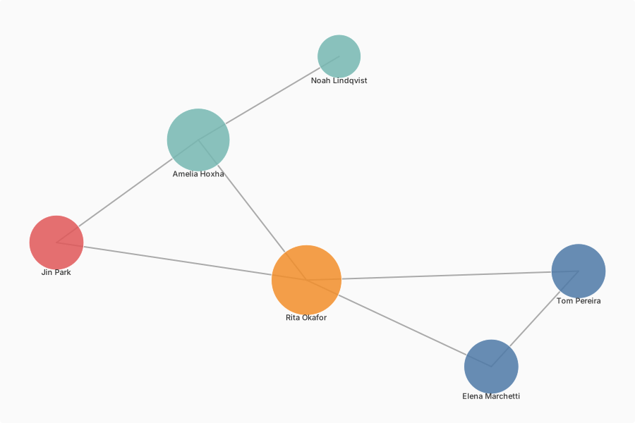
| Decade | Colour |
|---|---|
| 1960s | blue |
| 1970s | orange |
| 1980s | red |
| 1990s | teal |
Each node is sized by how many connections it has, so Rita and Amelia, who have the most knows edges, show up largest.
7. Filter on the derived field
where() filters by property value, and our new decade_born field is just another property, so we can filter on it directly:
Two people, with one knows edge between them.
8. Build a DataFrame and write a CSV
entity_records() returns a list of dictionaries (one per entity) that pandas understands directly:
import pandas as pd

df = pd.DataFrame(people.entity_records()).sort_values("birth_year").reset_index(drop=True)
df[["label", "birthDate", "birth_year", "decade_born"]].head()
             label   birthDate  birth_year  decade_born
0  Elena Marchetti  1962-03-04        1962         1960
1      Tom Pereira  1968-11-22        1968         1960
2      Rita Okafor  1975-07-09        1975         1970
3         Jin Park  1983-01-30        1983         1980
4     Amelia Hoxha  1991-05-17        1991         1990
The full DataFrame has every property as a column, plus four always-present columns at the front: id, label, type, and types. We're picking out four columns here just to fit the page; in a notebook, df.head() will show them all side by side.
Sorting by birth_year works because the values keep their natural Python types: birth_year is a real integer rather than a string, so pandas sorts it numerically rather than alphabetically.
If you prefer polars, the same list of records works with pl.DataFrame(people.entity_records()).
Saving to CSV is just pandas:
Next steps
There's a companion to entity_records() called relationship_records() that does the same thing for the edges. It's useful when you want a table of who-knows-whom or who-is-affiliated-with-whom. And once you've written a CSV, you can bring it back into Python at any point with pd.read_csv("people.csv") for further analysis.